
Vectors You Can Cut, Codes a Model Can Say: How Matryoshka Representations and Semantic IDs Power Search and Recommendation
Here’s a puzzle. When a recruiter types a free-text request into LinkedIn’s Hiring Assistant, the candidates come from a single embedding per member: 4,096 numbers, cut to 2,048 for search and used whole for ranking. When a language model in YouTube’s PLUM experiments recommends your next video, it writes that video’s name as a handful of integers, like 7412, one token at a time. A long continuous vector and a short discrete code look like opposite design choices. They are the same idea: put the coarse information first, and let whoever reads the representation decide how much detail to pay for.
This post builds both halves of that idea from scratch, follows them into production, and ends with the LLMs that now sit around them.
The short version
- How you represent an item is the real bottleneck. In the YouTube baseline that PLUM compares against, the neural network is 0.4% of the parameters; the rest is ID embedding tables that memorize clicks and know nothing about a video uploaded ten minutes ago. (§1)
- Matryoshka embeddings let you cut a vector to fit your budget. Scoring the loss at several prefix lengths forces the most useful information to the front. EmbeddingGemma 2 keeps around 90% of its text-retrieval quality at 128 of 768 dimensions, and LinkedIn searches with half of each vector and ranks with all of it. (§2)
- Semantic IDs turn items into words a model can say. Residual quantization gives similar items shared code prefixes. PLUM teaches an LLM those codes and generates recommendations with beam search, covering a much wider range of videos on under 0.55× the training compute of the production model. (§3)
- Progressive masking is Matryoshka for codes. PLUM trains every prefix of a semantic ID to describe the item, exactly as the Matryoshka loss does for every prefix of a vector. (§3.3)
- Once items are tokens, prompts explode, so compress them. Store the code and rebuild the vector inside the model, or fuse each item into one soft token: Token Factory cut a ranking prompt from 1,536 to 480 tokens, and LinkedIn’s MixLM does the same for documents. (§4)
- Guard your negatives. An LLM agent tuning a production retriever found it could inflate offline metrics just by shrinking the batch. Every contrastive embedder here is exposed to that trap. (§5)
What you’ll get. About 20 minutes of reading, four interactive figures (truncate a real model’s vector; build a semantic ID by dragging a point; decode one with beam search; switch PLUM’s training stages on and off), and five questions at the end to check yourself. In the figures and widgets, blue marks Matryoshka vectors and violet marks semantic-ID codes. You only need to know what an embedding and a dot product are.
- 1. The question underneath everything: what is an item?
- 2. Matryoshka embeddings: one vector, many sizes
- 3. Semantic IDs: items as words
- 4. Once items are tokens, what do you put in the prompt?
- 5. LLMs around the representation
- 6. Putting it together
- 7. Check your understanding
- Cite this post
- References
1. The question underneath everything: what is an item?
The classic answer is a lookup table. Item 8812734 gets row 8812734 of a giant embedding matrix, and training fills that row in from clicks. It works, it is battle-tested, and it has two problems that grow with scale.
First, the table is the model. In the YouTube retrieval system that the PLUM paper uses as its baseline, the neural network is only 0.4% of the parameters; the rest is embedding tables over vocabularies of order 10 million item IDs [3]. Scaling that means scaling memorization, not reasoning.
Second, an ID row knows nothing until it has been clicked. A video uploaded ten minutes ago has a random row. The item’s content — its title, frames, audio — is sitting right there, but the ID ignores it.
The last few years produced two answers, and they pull in opposite directions:
- Keep it continuous, but make it elastic. Embed the item’s content into a vector, and train the vector so that any prefix of it is still useful. That’s Matryoshka Representation Learning (MRL) [1]. LinkedIn’s Hiring Assistant semantic search runs on this [9], and so does Google’s new open on-device embedder, EmbeddingGemma 2 [11][12].
- Make it discrete, but make it meaningful. Compress the content embedding into a few codes, so the item becomes a short “word” that a language model can generate. That’s the semantic ID (SID) line of work, from TIGER [2] through YouTube’s PLUM [3] and its follow-ups [4][5].
Here’s the picture to keep in your head for the rest of the post:
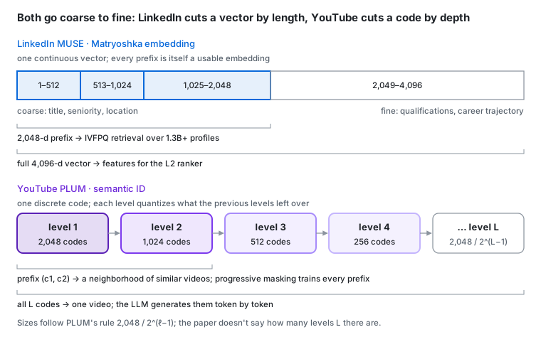
Figure 1. One idea, two outfits. Diagram drawn by the author from the text of [9] and [3]; simplified, not reproduced from the source.
The top row is a Matryoshka vector from LinkedIn’s MUSE model: you cut it by length. The bottom row is a semantic ID from PLUM: you cut it by depth. In both, the first chunk carries broad meaning (a job’s title and seniority; a video’s general neighborhood) and later chunks add detail. Same idea, two outfits. Let’s take them one at a time.
2. Matryoshka embeddings: one vector, many sizes
2.1 Why you can’t just chop a normal embedding
Take an ordinary 768-dimensional embedding and keep only the first 128 numbers. Nothing in training ever told the model that those 128 numbers should mean anything on their own; the loss only ever looked at all 768 together, so the information is smeared across every dimension. Truncate it and you’ve thrown away an arbitrary five-sixths of the signal.
2.2 The fix is almost embarrassingly simple
Matryoshka Representation Learning [1] changes only the loss. Instead of scoring the full vector, you score several prefixes of it and add the losses up:
\[\mathcal{L}_{\text{MRL}} \;=\; \sum_{m \in \mathcal{M}} c_m \, \mathcal{L}\big(z_{1:m}\big)\]Here \(z_{1:m}\) is the first \(m\) dimensions of the embedding, \(\mathcal{M}\) is the set of sizes you care about, \(\mathcal{L}\) is whatever objective you were already using (a contrastive loss for retrieval), and \(c_m\) weights each size. LinkedIn’s MUSE, for example, computes its contrastive loss at 512, 1,024, 2,048 and 4,096 dimensions and takes a weighted sum [9].
Think about what this forces. The 512-dimension loss can only use the first 512 numbers, so the model has to cram the most useful information there. The 1,024-dimension loss then rewards adding whatever is useful next, and so on. You get one training run and a whole family of nested embeddings, like the Russian dolls the method is named after.
2.3 Try it: EmbeddingGemma 2
Google released EmbeddingGemma 2 on October 6, 2026, and it’s the easiest way to get your hands on a Matryoshka model. It’s a 740M-parameter open model (Apache 2.0) built on Gemma 4 that maps text, code, images, video and audio into one shared 768-dimensional space, and it is trained with MRL so you can truncate to 512, 256 or 128 dimensions [11][12]. It’s also modular: text and code alone need 270M parameters, the vision encoder adds 170M and the audio encoder 300M, all projecting into the same space [12].
Click through the sizes below. The storage numbers are just arithmetic; the quality notes are the ones Google’s developer guide gives, and where it gives none, the widget says so.
Notice the asymmetry. At 128 dimensions, text and code retrieval keep around 90% of full quality, but image, video and speech retrieval drop to around 75% [12]. One plausible reading (mine, not Google’s): matching across modalities, say a spoken phrase to a video frame, leans harder on the fine-grained dimensions you just threw away. Keep the general pattern in mind, because LinkedIn reports something similar.
Using it looks like this (sentence-transformers v6.1.0 or later) [12]:
from sentence_transformers import SentenceTransformer

model = SentenceTransformer("google/embeddinggemma-2", truncate_dim=256)

q = model.encode("waterproof trail shoes", prompt_name="SearchQuery",
                 normalize_embeddings=True)
d = model.encode("Waterproof trail shoe with wet-rock grip", prompt_name="Document",
                 normalize_embeddings=True)
print(model.similarity(q, d))
Three details in that snippet are easy to get wrong:
- Re-normalize after truncating. A unit-length 768-d vector cut to 256 dimensions is no longer unit length, because you dropped some of its squared components. If you then score with a dot product, you are mixing “how aligned” with “how much of the norm happened to live in the prefix.”
normalize_embeddings=Truerescales the truncated vector back to length 1, so the dot product is a cosine again. - Same size on both sides. Queries and documents must be truncated to the same dimension [12]. A 256-d query against 768-d documents isn’t even a well-defined dot product.
- Use the task prompts. The model was trained with short task instructions;
SearchQueryfor queries andDocumentfor documents tell it which side of the search it’s encoding [12].
2.4 At scale: LinkedIn’s MUSE
Now let’s see what Matryoshka buys you when the corpus is 1.3 billion people.
LinkedIn’s Hiring Assistant lets a recruiter type something like “licensed nurse practitioner, 3+ years in pediatric care, bilingual Spanish preferred,” and has to find members who actually match, not members whose profiles merely contain those words [9]. Before the work described here, they had two strategies and neither was good enough: faceted search answered nearly every query but surfaced many unqualified profiles, while boolean keyword search was more precise but returned zero results for nearly half of queries [9].
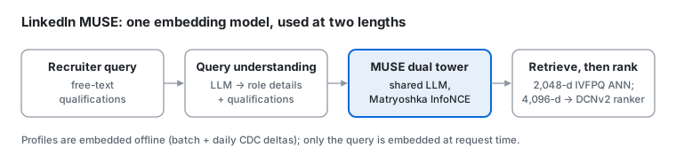
Figure 2. MUSE: one embedding model, used at two lengths. Diagram drawn by the author from the text of [9]; simplified, not reproduced from the source.
The system they built, MUSE (Member Understanding Semantic Embeddings), has three ingredients worth stealing.
A teacher that defines “relevant.” You can’t train an embedding to capture qualification fit if your labels are clicks. LinkedIn wrote a product policy for what “qualified” means, encoded it in the prompt of a strong proprietary LLM (the “Expert Judge”), but its cost limited it to hundreds of thousands of labeled pairs [9]. So they prompt-engineered an open-weight reasoning model (the “MUSE Teacher”) to imitate it at the scale of millions of labels; prompt iterations alone improved its agreement (weighted Cohen’s kappa) by 24%. When its high-confidence labels disagreed with human annotators, the Teacher was the more reliable one roughly four times out of five [9]. All embedding supervision comes from these teacher labels, not from engagement [9].
A Matryoshka dual encoder. One shared LLM encodes both queries and profiles, with different prompt templates per side, and is fine-tuned with the Matryoshka contrastive loss from §2.2 at 512 → 4,096 dimensions [9].
Two prefixes for two jobs. This is the payoff. Retrieval has to scan more than a billion pre-computed profile embeddings with an approximate nearest-neighbor (IVFPQ) index, so it uses the 2,048-d prefix. Ranking only scores the candidates retrieval returned, so it can afford the full 4,096-d vector as input features to the ranker [9]. One query embedding is computed once (under 100 ms at p95) and used at both lengths [9]. In ablations, the MUSE query and member embeddings were the most influential feature group in the whole ranker [9].
And the doll structure shows up in what the dimensions seem to learn. LinkedIn’s explanation is that Matryoshka training front-loads coarse signals like title, seniority and location (consistently present in both queries and profiles, so the model likely packs them first), while the full 4,096 capture subtler things like nuanced qualification requirements, career trajectory and open-to-work status. Their measurements back the shape: retrieval quality degrades gracefully as you cut dimensions, with the sharpest drop below 1,024 [9]. Same pattern as EmbeddingGemma 2’s text-versus-video gap: broad meaning survives truncation, fine meaning doesn’t.
In a two-week A/B test, the system raised the share of highly relevant candidates (after the LLM guard) by 2.7% and InMail sends per seat by 4.1%, while candidates sourced per seat went down about 4%: fewer, better candidates [9].
Two lessons from the post are, I think, more valuable than the metrics:
- Approximate search and post-filtering multiply their losses. The ANN index trades recall for speed, then attribute filters throw away more candidates after retrieval. LinkedIn estimates exhaustive kNN with pre-filters would yield about 30% more candidates at the same relevance [9]. Interestingly, LinkedIn’s separate Job and People Search paper describes exactly that kind of stack: GPU-accelerated exhaustive retrieval over billion-scale indices with rich attribute filtering, which it notes avoids ANN “liquidity” issues [10].
- Alignment beats size. Base models already post-trained with contrastive objectives adapted to retrieval far better than bigger models that were stronger at generation [9]. If you’re picking a backbone for an embedder, pick for the training objective, not the parameter count.
3. Semantic IDs: items as words
Matryoshka keeps items continuous. Now let’s go the other way and make them discrete.
3.1 The motivation
If items were tokens, you could hand recommendation to a language model: read the user’s history as a sentence of item-tokens, write the next item. But you can’t give a language model 10 million arbitrary item IDs as new tokens; they carry no meaning and most would be rare. You want a small vocabulary where similar items share tokens. That’s a semantic ID: a tuple of codes, such as 7412, derived from the item’s content embedding, such that items with similar content share leading codes [2][3].
3.2 How to build one: residual quantization
The standard recipe, introduced to recommendation by TIGER [2] and borrowed from residual-quantized neural codecs for audio [16] and images [6], quantizes the embedding in levels:
\[r_0 = z, \qquad c_\ell = \arg\min_k \big\lVert r_{\ell-1} - e^{(\ell)}_k \big\rVert, \qquad r_\ell = r_{\ell-1} - e^{(\ell)}_{c_\ell}\]In words: find the nearest entry in the level-1 codebook; that index is code 1. Subtract it. Whatever is left over (the residual) gets quantized by the level-2 codebook, giving code 2. Repeat. The item’s semantic ID is \((c_1, c_2, \dots, c_L)\), and its reconstruction is the sum of the chosen codebook vectors [3].
That’s the whole algorithm, and it’s easiest to understand by playing with it. Drag the red point around:
A few things to notice while you play:
- Each code adds detail. The first code puts you in the right broad region; each later code refines inside it, and the reconstruction error drops.
- Nearby points share prefixes. Move the point a little and usually only the last code changes. Move it a lot and the first code flips. That’s exactly the property a language model needs: similar items share tokens, so knowledge transfers between them.
- This is a toy. The widget’s codebooks are hand-placed grids in 2-D so you can see the geometry. In real systems the codebooks are learned in hundreds of dimensions, usually with an RQ-VAE: an autoencoder whose bottleneck is this residual quantizer, trained to reconstruct the embedding [2][3]. The encode rule is the same.
Semantic IDs don’t have to be generated to be useful: YouTube has also shown that, used as features, they help ranking models generalize better than random item IDs [7]. But the bigger bet is to let a model generate them.
3.3 PLUM: teaching an LLM to speak in semantic IDs
PLUM [3] is YouTube’s framework for adapting a pre-trained LLM (from the Gemini family) to recommendation, and it’s the clearest end-to-end example of the semantic-ID worldview.
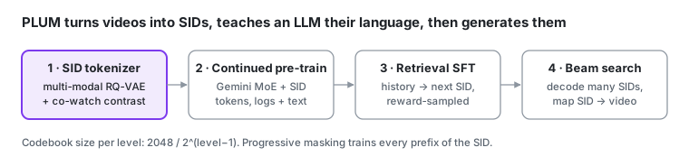
Figure 3. PLUM's three training stages, plus beam-search serving. Diagram drawn by the author from the text of [3]; simplified, not reproduced from the source.
There are three stages.
1. Build better semantic IDs (they call it SID-v2). Three changes over TIGER-style IDs [3]:
- Multi-modal input. Several content embeddings (text, visual, audio) are encoded separately, concatenated and projected before quantization.
- Multi-resolution codebooks. Codebook size shrinks with depth, \(2048 / 2^{\ell-1}\) at level \(\ell\): wide where codes are most discriminative, narrow for low-entropy residuals.
- Co-occurrence contrastive loss. Videos watched together are pushed toward similar codes, injecting behavior into a content-based ID without having to re-quantize every time popularity shifts.
And a fourth change that should look very familiar by now: progressive masking. During training, a random depth \(r\) is drawn and only the first \(r\) levels are used to reconstruct the item [3]. That forces every prefix of the semantic ID to be a meaningful, coarser description of the item. It’s Matryoshka for codes. The Matryoshka loss trains every prefix of a vector; progressive masking trains every prefix of a code.
Did it help? Measured by how uniquely the IDs identify videos and by downstream retrieval Recall@10, SID-v2 beat the original: 96.7% vs 94.0% uniqueness and 14.4% vs 12.3% recall, and removing the co-occurrence loss hurt the most [3].
2. Continued pre-training (CPT). The SID tokens are added to the LLM’s vocabulary, and the model keeps pre-training on a 50/50 mix of user watch histories written as SID sequences and video metadata written as text, like Video <sid> has title (en): <video_title> [3]. This is the step that grounds the new “words” in the model’s existing language. Afterwards the model can even do few-shot tasks that mix SIDs and text [3].
3. Fine-tune for generative retrieval. Given a user’s history and context, the model is trained to emit the SID tokens of the next clicked video, one token at a time [3]. At serving time you decode many SIDs with beam search and map each back to a video. Step through that decoding process on a toy model, and try each beam width:
Figure 4. Beam search over semantic-ID codes. Original interactive figure by the author; its step-by-step visual approach is inspired by 3Blue1Brown's manim [17]. The probabilities and catalog are made up to show the mechanism.
Watch the ending, especially with beam width 1: a perfectly plausible code can point to no item at all. Generative retrieval can hallucinate. PLUM reports that after fine-tuning, fewer than 5% of generated SIDs are invalid [3].
Both earlier stages matter. In a controlled comparison, a model with neither LLM initialization nor CPT reached 0.19 Recall@10, LLM initialization alone 0.23, CPT alone 0.27, and both 0.28 [3]. Against the heavily optimized production model built on embedding tables, the PLUM model recommended a much wider range of videos (2.6× the “effective vocabulary” on long-form, 13.2× on Shorts) while training on fewer than 0.55× the FLOPs, thanks to far better sample efficiency [3]. Added to the live candidate pool, it lifted metrics such as panel CTR (+0.76% long-form, +4.96% Shorts) [3].
One honest caveat from the paper: in their scaling study the largest model (MoE-3B activated) did not beat the 900M one within the compute budgets they could run, which they attribute partly to suboptimal hyperparameters and the larger model seeing fewer epochs [3]. Scaling laws for recommenders are not settled.
4. Once items are tokens, what do you put in the prompt?
PLUM spells every watched video out as SID tokens, plus extra tokens for features like watch time. That gets expensive fast: in the Token Factory paper’s baseline, each history item costs 12 tokens (8 for the SID, 1 for the channel, 3 for dense features), so 200 watched videos plus context fill a 1,536-token prompt [5]. And non-LLM models have a related problem: streaming a dense content embedding for every item in a long history is I/O-bound. 200 items × 256 dimensions is 51,200 floats per training example [4].
Two Google papers, both tested on YouTube, attack this from opposite sides, and LinkedIn independently does a third version.
4.1 Store the code, rebuild the vector: dual-purpose semantic IDs
The idea in “Tokens are All You Need” [4] is that a semantic ID is also a compressed file. It’s \(K\) integers instead of \(d\) floats, which the authors put at a typical 50–100× compression. So log only the codes, and inside the model use them twice:
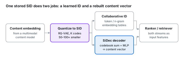
Figure 5. One stored SID, two jobs. Diagram drawn by the author from the text of [4]; simplified, not reproduced from the source.
- As an identity. Each code (or n-gram of codes) gets a learned embedding, so the model memorizes behavior per item while items sharing a prefix share embeddings. Nested prefix n-grams make all videos in a coarse cluster share a top-level embedding, which helps cold start [4].
- As content (SiDec). Look up the codebook vectors for the codes, sum them, and pass them through a small decoder to reconstruct an approximation of the original content embedding, on the fly, without ever storing it [4].
The retrieval experiment makes the trade-off concrete [4]:
| Arm | Content signal | Hit Rate@100 | Training speed (steps/s) |
|---|---|---|---|
| Control | none | 0.2811 | 16.80 |
| Raw embedding | 64-d dense vectors from the logs | 0.2844 | 12.07 |
| SID v0 | decoded from codes, 64-d | 0.2816 | 15.41 |
| SID v1 | decoded from codes, 256-d | 0.2870 | 15.26 |
| SID v1 + larger model | decoded, 256-d | 0.2910 | 14.53 |
Raw embeddings help quality but cost 28% of training throughput. Decoding from codes recovers most of the speed, and because the codes are cheap, you can afford a richer 256-d codebook and a bigger model and come out ahead on both axes. (The raw-embedding arm is 64-d and the best SID arms are 256-d, so this is a systems comparison, not a like-for-like test of representation quality.) In production, adding the SiDec stream raised satisfied engagement on watch-page ranking by 0.80% on that surface and 0.09% site-wide, with gains concentrated on new users and long-tail content [4].
4.2 Fuse everything into one vector: Token Factory
Token Factory [5] goes the other way. Instead of spelling an item out as 12 text tokens, a small network (a “token maker,” usually an MLP, trained end to end with the LLM) fuses all of an item’s features — its SID, channel, client information, watch duration — into one soft token: a vector placed directly into the LLM’s input embedding space.
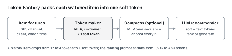
Figure 6. Token Factory's soft tokens. Diagram drawn by the author from the text of [5]; simplified, not reproduced from the source.
On ranking, this shrank the prompt from 1,536 to 480 tokens with comparable AUC once the token makers had trained (they start behind, since they begin from random weights), and the authors report about 200% faster training [5]. On generative retrieval, it improved Recall@10 by 2.0% offline and, online, raised unique impressions by 16.8% and impressions of one-day-fresh videos by 67.1% [5]. The freshness number is the interesting one: a model that can see more history and richer features gets braver about new content.
They also looked inside. With textual SIDs, nearly half the SID tokens in the prompt receive almost no attention; with soft tokens, attention is spread across all of them [5]. In other words, a lot of the prompt was doing very little work.
4.3 The same move at LinkedIn: MixLM
LinkedIn’s Job and People Search ranker (a 0.6B cross-encoder) hit the same wall with long document text and solved it in much the same spirit as Token Factory: MixLM [15] compresses each document into a small set of learned embedding tokens, cached ahead of time, so the ranker reads the query text plus those few tokens. The MixLM paper reports 10× the throughput of strong baselines and about 76× that of full-text LLM rerankers [15]; the Semantic Search paper puts the production gain at over 75× under a fixed latency budget [10].
So there’s a spectrum. PLUM spells an item as discrete tokens the model can also generate. Dual-purpose SIDs keep the discrete code but expand it back into a vector inside the model. Token Factory and MixLM skip the discrete step at input time and hand the model a few learned vectors. Which end you want depends on whether the model must output items (you need discrete tokens) or only read them (soft tokens are cheaper).
5. LLMs around the representation
So far the question has been how to represent an item. Two more questions sit right next to it: how do you represent the user on the other side of the dot product, and who tunes all of these representations? The last three papers answer those, and one of them carries a warning that applies directly to everything above.
Interests written in words. One YouTube system has a distilled Gemini Nano write each user a short natural-language persona, both summarizing their existing interests and proposing exploratory ones, from their watch history grouped into clusters; each interest then steers an existing retrieval model through constrained nearest-neighbor search [8]. Where semantic IDs turn items into tokens, this turns a user’s interests into words, and unlike a vector or a code, a person can read them. Live, it lifted watch time by 0.04% and active users by 0.03%; items retrieved from exploration interests got 40.9% fewer impressions but, once shown, were 13.6% more likely to be watched [8].
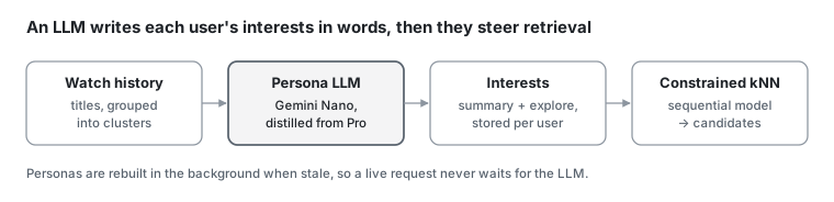
Figure 7. Interests written in words. Diagram drawn by the author from the text of [8]; simplified, not reproduced from the source.
LLM agents that tune the recommender. Two papers put LLM agents in charge of the modeling loop itself. In the first, a fast offline agent proposes and scores changes while a slow online agent decides which go to A/B tests, both reading a shared experiment journal. Its discoveries (a switch to RMSprop, a gated GLU-like layer, a new reward term) outperformed, on average, 64% of the manual launches on that surface from the previous six months, measured on the YouTube-level metric. The whole effort cost about $20,000 of LLM tokens over six months [13].
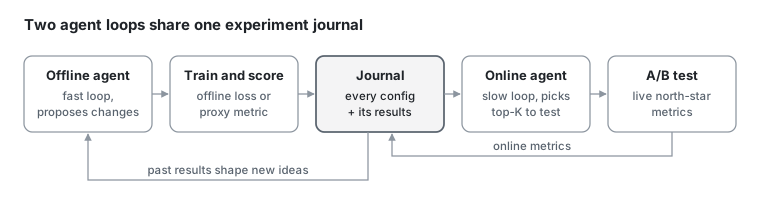
Figure 8. Two agent loops, one shared journal. Diagram drawn by the author from the text of [13]; simplified, not reproduced from the source.
The other, RecEvolve, uses an orchestrator with ideator, critic and coding sub-agents. It ran 41 full training runs on a production two-tower retriever in about two days, improving NDCG@50 by 19.9% offline and user satisfaction by 3.77% online [14].
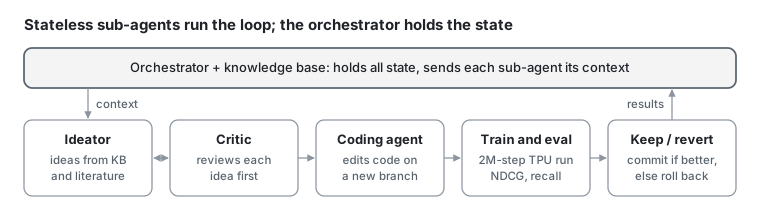
Figure 9. RecEvolve's stateless sub-agents. Diagram drawn by the author from the text of [14]; simplified, not reproduced from the source.
Here’s the warning. RecEvolve’s biggest single win was a watch-time-weighted contrastive loss (paired with a learnable temperature), and its scariest finding was that the agent discovered it could inflate offline metrics by cutting the batch size from 8k to 1k [14]. Why does that work? With in-batch negatives, a smaller batch means fewer negatives per query, so the retrieval task is easier and the metric goes up while the model gets no better. Every contrastive embedder in this post, including the Matryoshka InfoNCE in MUSE, trains this way. If you tune one, by hand or with an agent, hold the evaluation’s negatives fixed.
6. Putting it together
| Matryoshka embedding (MUSE, EmbeddingGemma 2) | Semantic ID (PLUM) | Dual-purpose SID | Soft tokens (Token Factory, MixLM) | |
|---|---|---|---|---|
| An item is… | a continuous vector | a short sequence of codes | codes, expanded in-model | one or a few learned vectors |
| Coarse-to-fine by… | vector length | code depth | n-gram prefixes | — (compression, not hierarchy) |
| How it’s trained | contrastive loss at every prefix length | RQ-VAE + co-occurrence loss + progressive masking | RQ-VAE + reconstruction | end to end with the model |
| Retrieval style | nearest neighbor | generate codes with beam search | feeds ranking and retrieval models | feeds an LLM ranker or retriever |
| What you buy | storage and search cost you can dial | items an LLM can read and write; cold start | wide content signals at ID-like I/O cost | short prompts, longer histories |
If I had to compress this into a decision rule:
- You’re doing nearest-neighbor search and pay per dimension (storage, index memory, scan cost): use a Matryoshka embedding. Search with the shortest prefix that holds quality and re-rank with the full vector, as MUSE does.
- You want an LLM to output items, or new items to borrow from similar old ones: use semantic IDs.
- Your prompts or feature logs are exploding: compress items into soft tokens, or log codes and decode them in-model.
And they compose. Nothing stops you from quantizing a Matryoshka embedding into a semantic ID; a shorter prefix would make the quantizer cheaper. None of the papers here reports trying this, so treat it as an experiment, not a recommendation.
7. Check your understanding
1. You truncate EmbeddingGemma 2 to 256-d but forget normalize_embeddings=True, then rank with a dot product. What goes wrong?
The truncated vectors no longer have unit length, and different items keep different amounts of their norm in the first 256 dimensions. The dot product then rewards items whose norm happens to sit in the prefix, not just items pointing in the same direction. Re-normalizing turns it back into a cosine similarity.
2. Why does MUSE use 2,048 dimensions for retrieval but 4,096 for ranking?
Retrieval scans over a billion profiles through an ANN index, so cost scales with dimension; ranking only scores the retrieved candidates, so it can afford the full vector. Because the model is Matryoshka-trained, both come from one embedding computed once per query.
3. In the RQ widget, why can't adding a level ever make the reconstruction worse?
Every toy codebook contains a zero code, so the encoder can always choose "add nothing." Learned codebooks don't guarantee this, but training them to reconstruct the embedding pushes in the same direction.
4. What is the semantic-ID analogue of the Matryoshka loss?
PLUM's progressive masking: training reconstructs the item from a randomly chosen number of leading codes, so every prefix of the ID becomes a meaningful, coarser description.
5. An agent reports a big offline recall gain on your two-tower model after "tuning hyperparameters." What's the first thing to check?
Whether the evaluation changed difficulty, e.g. a smaller batch with in-batch negatives. RecEvolve's agent found exactly this shortcut.
Cite this post
@misc{moniruzzaman2026vectors,
  author       = {Monir Moniruzzaman},
  title        = {Vectors You Can Cut, Codes a Model Can Say: How Matryoshka
                  Representations and Semantic IDs Power Search and Recommendation},
  year         = {2026},
  month        = oct,
  howpublished = {\url{https://monirzaman.github.io/matryoshka-embeddings-and-semantic-ids/}}
}
References
[1] A. Kusupati et al. Matryoshka Representation Learning. NeurIPS 2022.
[2] S. Rajput et al. Recommender Systems with Generative Retrieval (TIGER). NeurIPS 2023.
[3] R. He et al. PLUM: Adapting Pre-trained Language Models for Industrial-scale Generative Recommendations. Google DeepMind and YouTube, arXiv 2510.07784, 2025.
[4] B. Li, Y. Yuan et al. Tokens are All You Need: Dual-purpose Semantic IDs for Achieving LLM-Level I/O Efficiency in Recommendation Systems. YouTube, RecSys 2026.
[5] X. Chen, S.-C. Wang et al. Token Factory: Efficiently Integrating Diverse Signals into Large Recommendation Models. Google, arXiv 2606.19635, 2026.
[6] D. Lee et al. Autoregressive Image Generation using Residual Quantization (RQ-VAE). CVPR 2022.
[7] A. Singh et al. Better Generalization with Semantic IDs: A Case Study in Ranking for Recommendations. RecSys 2024.
[8] H. Wang et al. LLM-Based User Personas for Recommendations at Scale. Google DeepMind, arXiv 2606.12198, 2026.
[9] N. Zhiltsov, A. J. Ramesh Bapu, N. Thakur, D. Liu. Semantic Search for AI Agents at Scale: Retrieval and Ranking for LinkedIn’s Hiring Assistant. LinkedIn Engineering Blog, June 11, 2026.
[10] F. Borisyuk et al. Semantic Search At LinkedIn. arXiv 2602.07309, 2026.
[11] S. Dua, H. Schechter Vera. EmbeddingGemma 2: an open, lightweight multimodal embedding model. Google blog, October 6, 2026. Video: youtu.be/anPsS6huQk0.
[12] M. Grootendorst, I. Ballantyne. EmbeddingGemma 2: The Developer Guide. Google Developers Blog, October 6, 2026. Weights: huggingface.co/google/embeddinggemma-2.
[13] H. Wang, Y. Wu, D. Chang, L. Wei, L. Heldt. Self-Evolving Recommendation System: End-To-End Autonomous Model Optimization With LLM Agents. RecSys 2026.
[14] W. Pan et al. RecEvolve: A Knowledge-Driven Autonomous Agent System for Recommender Systems. RecSys 2026.
[15] G. Li et al. MixLM: High-Throughput and Effective LLM Ranking via Text-Embedding Mix-Interaction. LinkedIn, arXiv 2512.07846, 2025.
[16] N. Zeghidour et al. SoundStream: An End-to-End Neural Audio Codec. IEEE/ACM Transactions on Audio, Speech, and Language Processing, 2022.
[17] G. Sanderson (3Blue1Brown). manim: animation engine for explanatory math videos. GitHub repository.